My Credentials:

About the Snowpack Model

The model tries to predict recent additions to the snowpack on Sasse Ridge as inches of new snow from top to bottom.

Foolish as this is, it worked better than I might have expected over the last winter.

Why inches and not SWE? Because I'm a skier; that's what a skier wants to know!

The resulting charts only cover the past week.

Inputs

The disadvantage of SWE data is that if the temperature at the Snotel site above freezing, precip will not be detected properly and the possibility of snow higher up will be discounted.

The simplifying assumptions are:

- that during periods of precipitation, the airmass in the local area is relatively homogeneous and that the amount of precip is the same at all elevations covered by the model. (Drastic, yes!)

- that during periods of precipitation, the temperature on Sasse Ridge drops roughly by the environmental lapse rate taken from soundings at Stampede Pass

- that precipitation will fall as snow and accumulate when the air temperature is below about 32 degrees (this value can be tweaked in the model)

- that a change in the precip counter followed in the next hour by an opposite but matching change is an aberration and represents no change

- that the precip counter is incremental; the values should not decrease. Nonetheless, during periods without precip the baseline often wanders up and down. For each data reporting period, the model checks the values for the preceding 12 hours and uses the maximum if it is higher

The most important assumption:

Two major issues that the model must address:

The Problem of Snow Density

The simplest solution is to use the ’ten to one’ rule;

- one inch of snow per tenth inch of precip, regardless of temperature. Not very realistic!

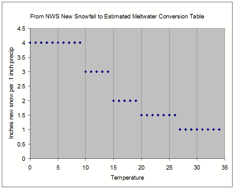
Another solution is to use the National Weather Service New Snowfall to Estimated Meltwater Conversion table. For every tenth inch precip, the table estimates the new snowfall as follows:

Graphed, it looks like this:

This may be a better solution, but it requires a lot of work to implement, and it’s still incremental.

Also, since temps on the valley floor are often near freezing, estimating an inch of new snow per inch at a temp of 34 degrees will lead to significant errors.

The model currently uses a power function times a multiplier with easily adjustable constants:

Expressed as snow density vs. temperature:

The lapse rate problem:

Originally the model assumed that during periods of precip, the temperature decreased with increasing elevation by the wet adiabatic lapse rate - 3 degrees per 1000 feet.

Instead of this theoretical value, the model now uses data from NWS radiosonde launchings at Stampede Pass.

The balloons report temperature and elevation at close increments up to ~60,000 feet.

The model uses only data up to about 8000 feet.

It generates a best-fit line through the data points and calculates the environmental lapse rate in degrees per 1000 feet.

An example:

Although the balloons are only launched twice a day, the NOAA Forecast Systems Laboratory provides forecasts /predictions for each hour of the day, including retrospective forecasts.

The model uses these hourly predictions when it processes the hour by hour Snotel data.

How the model works:

It’s just a large Excel file with several macros controlled by a Windows script for automation.

It calls up Snotel data from the web and with the hourly temperature from the site it predicts the temperature at 500 foot increments of elevation starting at the parking lot.

It uses the predicted temperature and the increase in precip since the last data period to estimate the amount of new snow for each of these elevations based on the assumptions above.

If the precip values are suspect, such a decrease in the value, the value is corrected using 'if-then' logic rules. The data for each hour reported from the site are similarly processed.

Excel then creates four different charts:

Chart 1:

a bar graph with bars for the different elevations.

In each bar colored segments represent snow that accumulated during a 2 hour interval. (One hour intervals too cumbersome)

The newest additions to the snowpack are on top.

The bar graph does not account for melting, compression, snowpack aging or wind transport, so the bars are not really virtual snowpits – but it's an easy way to think of them.

An example:

Chart 2:

the rate of accumulation of new snow at 3 different elevations for the previous week. This can be another useful tool in accessing avalanche danger.

An example:

Chart 3:

the total snow accumulated during each 2 hour interval for the past week. It also shows the solar radiation, and the barometric pressure.

An example:

The solar radiation values are useful for cross checking. Bright sun and lots of new snow at the same time suggest a problem!

Chart 4:

an attempt to predict the spring snowpack

Snotel Precipitation Sensor Issues

Snotel SWE and precipitation sensors are intended for water resource management and not for following hour by hour changes to the snowpack. With some discretion however, the sensors can provide surprisingly accurate near term information.

The snowpack model can use either SWE or precip as input, however SWE has several disadvantages:

• if it is raining at the Snotel site, it may be snowing above, and the sensor will miss some or all of this precip as the water drains out of the snow
• if rain soaked snow is later frozen hard by cold weather, the pressure from new snow on top may not be properly transmitted to the pillow below
• the SWE pillow may also be affected by snow creep
• because the snowpack is relatively firm, the pressure from new snow may take awhile to be transmitted down to the pillow (Last December, the lag was sometimes 4 hours.)

The snowpack model uses precip sensor data unless it is obviously wrong.

The precip gauge has limitations too.

Precip gauge errors other than major mechanical or electrical failure:

Taken from the Snotel sensor related web pages by Prof. Mark Williams and by Randall Julander, NRCS Water Supply Specialist:

http://snobear.colorado.edu/Markw/SnowHydro/Measuring_Snow/Snotel/snotel.html

http://www.civil.utah.edu/~cv5450/snotel/standards.htm

(These pages also discuss SWE pillows in detail.)